Perception, Localization, Planning and Control on RAE Robots

R. den Braber, M. Nulli, D. Zegveld

Intelligent Robotics Lab, University of Amsterdam

Links: 📝 Blogpost | 🧑‍💻 Code 1, 2, 3

Introduction

In this blogpost we go over our process of building an integrated perception–localization–planning–control pipeline on the RAE robot. Below we go over Camera Calibration and Line Following, Localization and Curlying Match playing (see Video 1) and Mapping, Planning and Control, to allow our RAE Robot to freely move across our environment.

Video 1: RAE Robots playing a Curlying Match with our Algorithms.

Camera Calibration and Line Following

In this section we demonstrate the effectiveness of our line-following pipeline by using a RAE robot to move parallel to the lines spanned by ceiling lights.

We began with camera calibration, which is shown to reduce distortion resulting in improved navigation accuracy. We do so comparing two algorithms of differing complexity, ultimately using Zhang’s [1] camera calibration technique.

Thereafter we developed a line‑following algorithm.

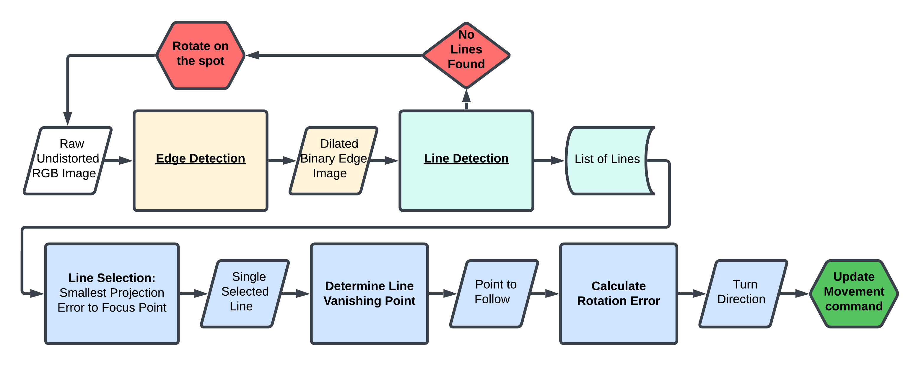
Figure 1: Overview of the full pipeline, where the lower blue part specifically covers the Line Selection and Line Following procedure. With the output of the Line Following procedure a Movement Update is calculated to direct the robot along the direction of the ceiling lights. Additionally, when no lines are detected the RAE robot is instructed to spin around until it finds the wanted ceiling lines (here in red).

First step is edege detection through an optimized version of the Canny edge detection algorithm. The next step is line detection, whose aim is to return a list of all lines that are spanned by the ceiling lights. It leverages a fine-tuned version of the Hough transform in addition to our triangular region of interest see blue line in Figure 2. Both the edge and line detection stages are refined by tuning the parameters and by adding additional steps such as image dilation to make the ceiling lines more prominent in the resulting image. This increases the robustness of our algorithm so that it can properly detect lines in difficult conditions, for example, at different angles, lighting conditions, and deal with gaps between the ceiling lights.

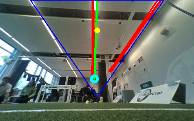
Figure 2: Displays a visualization of the output of the full pipeline. Here the blue triangle indicates our triangular region of interest. Red lines are candidate lines, while the green line is the selected line to follow. This line is determined to the the closest line to the focus point (yellow). At the endpoint of this line do we find the lines vanishing point (cyan) towards which the robot is steered..

Lastly, the line-following algorithm implements a way to consistently select the closest line, which removes the distraction of multiple detected lines. Next, using the selected line, we calculate a vanishing point to move towards instead of blindly following the line as this proves to increase navigational consistency and accuracy see Figure 2. Additionally, in an ablation study we found that utilizing this vanishing point approach allows our robot to still perform well, even without camera calibration, with only a slight potential reduction in navigational accuracy. This robustness highlights the strengths and adaptability of our pipeline (see Figure 1) which results in a stable and accurate ceiling light line following algorithm for the RAE robot.

Localization and Curlying Match

In this chapter we go over our setup for localization and curling match playing with the RAE robot, see Figure 3.

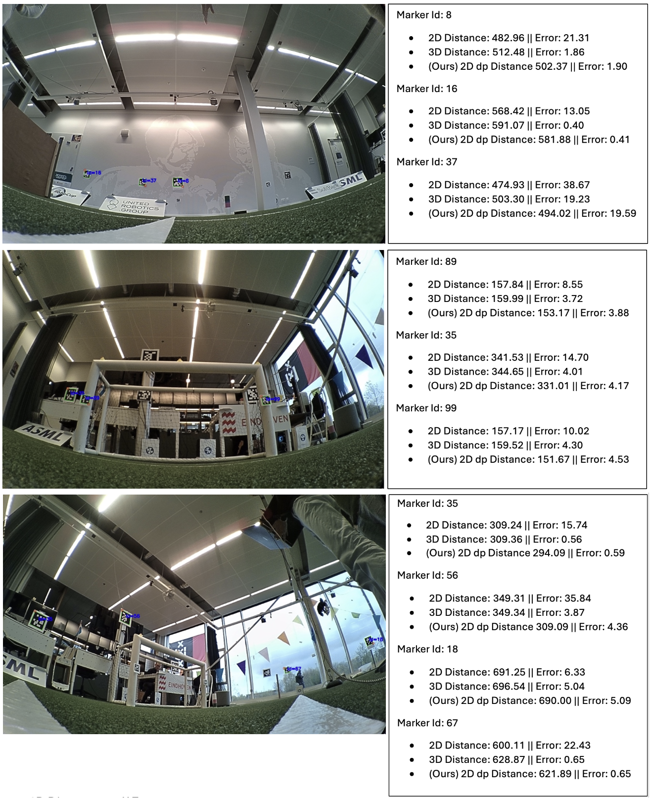
Figure 3: Curlying Match with our Algorithms. In these two videos we show the accuracy of our Localization Algorithm over multiple runs and multiple points of references.

We start by performing marker detection on QR-style code markers from APRILTAG. After improving our marker detection algorithm, we localize ourselves in real-world coordinates using the center of the field as the (0, 0) point. We consider different distance measurements and locate ourselves based on two, three, or more markers. Our marker-based localization algorithm allows us to obtain an average localization error of less than 13 cm, see Figure 4.

We utilize an Extended Kalman Filter [2] to merge our marker-based localization with the odometry motor-based estimated position to achieve a more accurate and robust location estimate during the match, see Figure 3.

Figure 4: Results on distance measurements from RAE Robot to Markers. We report the results of measurements for three different positions on the field. For each, we note the Marker ID, the three estimated distances, and the errors with the correct distance. The 2D Distance || Error represents the error between the 2D Distance from the camera of the robot and the marker and the corresponding error with the 2D correct distance. The 3D Distance || Error are the result of the 3D distance estimated through the cv2.solvePnP function and its error with the actual 3D distance to the marker. Lastly, the version we employ is the (Ours) 2D dp Distance || Error, which stands for the 2-dimensional down-projected distance of the above 3D and its error compared to the 2D correct distance.

Lastly, we design an algorithm which combines (Figure 5. ) a feature-based and position-based solution to ensure accurate and robust localization during the curling match. Furthermore, we incorporate object avoidance to navigate around other RAE robots that may block the path to the target location. Our algorithm achieves effective results through the coordination of three key nodes:

Localization node: Estimates the robot’s position using the detected markers.
Driving node: Uses motor-based odometry to estimate the robot’s position and combines it with marker-based localization in order to navigate toward the target location.
Object avoidance node: Signals when an object is in the way and identifies where in the image this object is to ensure that it is avoided (see the next section for more details).

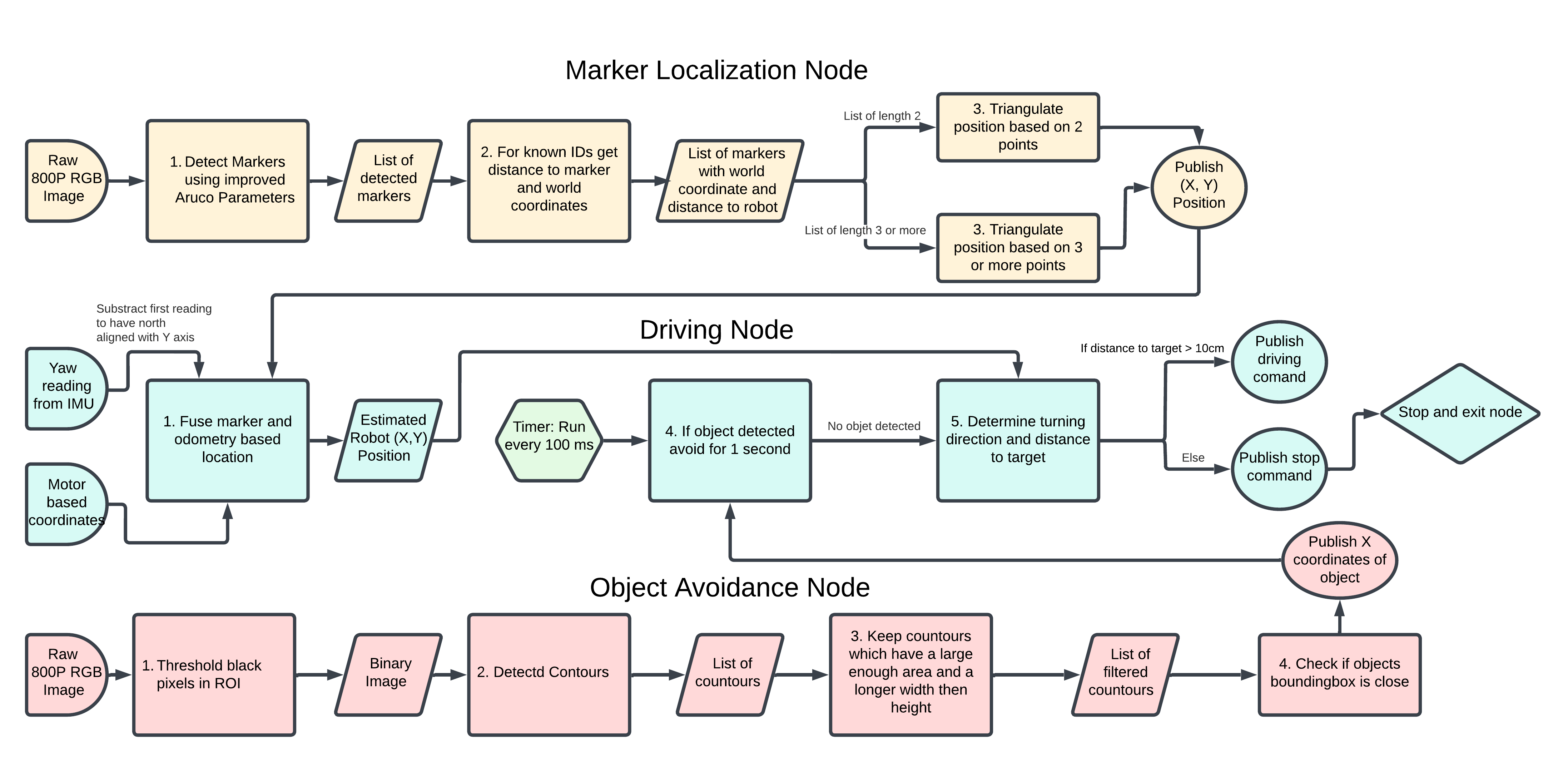
Figure 5: Full flow. The full pipeline for playing curling, with each node represented in a distinct color. Nodes subscribe to various RAE robot topics, shown as squares with rounded right edges, and also subscribe to topics published by other nodes, depicted as circles.

The visual marked-based localization works as described above and publishes the current location estimate of the robot as a point on a ROS topic. The driving node picks up this topic and combines it with its motor-based odometry using an EKF. For the driving node, we implemented the motor-based odometry by hand as we ran into some curious issues when trying to center the robot’s position using the built-in odometry implementation. This built-in implementation used an EKF as well between the motor-based odometry and the Inertial Measurement Unit (IMU), but upon resetting the starting location of the robot to (0,0) the IMU would behave erratically and report weird headings with a large error from the actual heading. For our implementation, we make use of the heading (yaw) reported by the IMU. However, before every run, we automatically reset the heading to 0 (north) by reading the initial IMU yaw value and subtracting this value from all further IMU readings. Now we can rely on the reported fixed headings, we also need to localize in cases where no visual localization is provided due to not detecting markers. We do this by subscribing to the motor odometry topic. This topic publishes the robot’s location as (x,y) coordinates from its internal reference frame based on the motor odometry. However, we want the (x,y) position in our real-world coordinate frame. To obtain this we calculate the distance that the robot drives by calculating the Euclidean distance between two (x,y) coordinate points from the last 2 consecutive motor odometry messages. We then use our heading theta to calculate the robot’s (x,y) position in our real-world coordinate frame using

x += \cos(\theta) \cdot (distance \ driven) and y += \sin(\theta) \cdot (distance \ driven)

Since we now have both the motor-based odometry location and the marker-based visual location, we combine these two with an EKF to create a more accurate, reliable, and robust prediction of our robot’s real-world location. This process, partially outlined in Section 2.5, is further clarified below. For both the odometry- and marker-based locations we use a different uncertainty matrix. For the marker location, we use an uncertainty matrix with a 13 cm standard deviation, this value corresponds to the average marker-based localization error that we found over a wide range of field positions, with different numbers of markers detected at different distances. The uncertainty matrix for the motor-based odometry uses a standard deviation of 20 cm, expressing the average error we measured after driving to different target locations relying solely on the motor odometry.

Given the reliable prediction of our world location and our known (improved) heading readings, we now have the information to navigate toward the real-world coordinates of the target location. We achieve this by calculating the required heading to drive from our current estimated location to the target location. Then we calculate the smallest angle between the current heading and the required heading and determine the direction in which to turn our robot by looking at the sign of this resulting angle. Furthermore, the rotation speed is determined by scaling this angle (in radians) with a gain factor, resulting in slower turns for smaller corrections. Lastly, the forward driving speed is calculated based on the distance to the target location, with a capped maximum speed limit. This similarly to the angle case, ensures more precise movements as the robot approaches the target location.

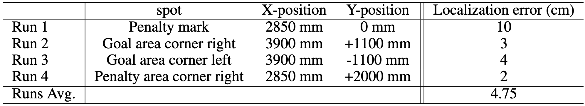
With the full pipeline active, the robot is able to drive towards all 5 target locations reliably, and can accurately localize itself from any starting position on the field using the detected markers, see Table 1.

Table 1: Curling Match Results: We report the results of the curling match performed on 4 different runs. For each run we had a different starting order, meaning that in most runs there already were robots positioned on the field. We show the spot that we are driving to, its coordinates (X-position, Y-position), together with the absolute distance from our finishing position to the target point Localization error (cm) in centimeters.

Mapping, Planning and Control

Finally we report the process of mapping and finding a path through a maze using only the video stream as captured with the RGB camera off the RAE robot.

First we create a 3D point cloud is created through Structure from Motion (SfM) and optimize it with COLMAP [3], see Figure 6.

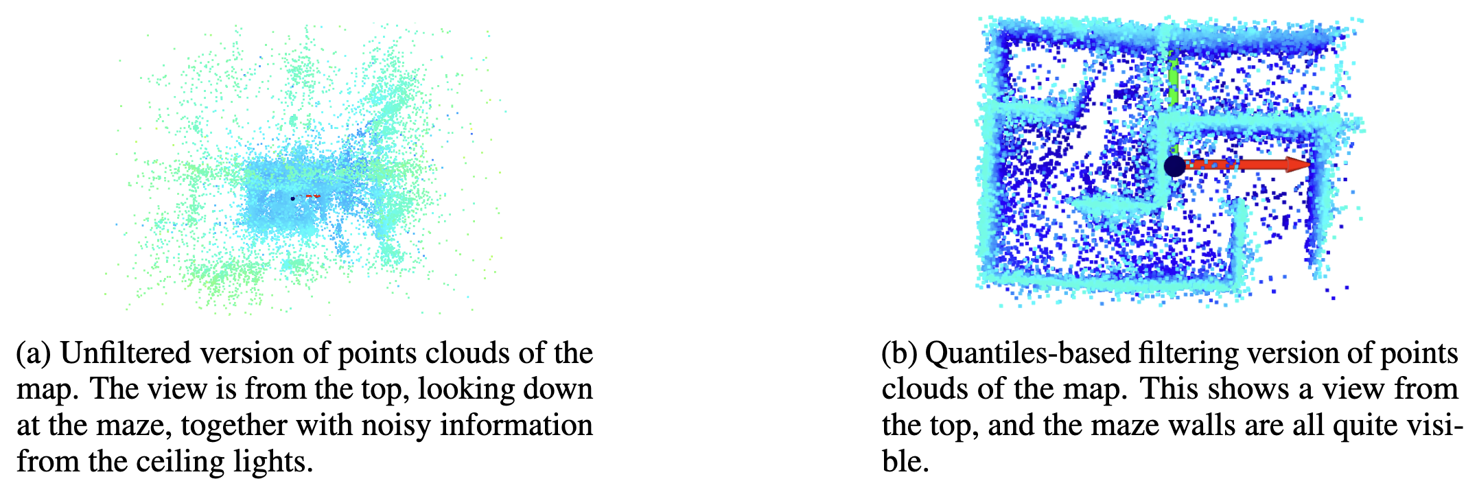
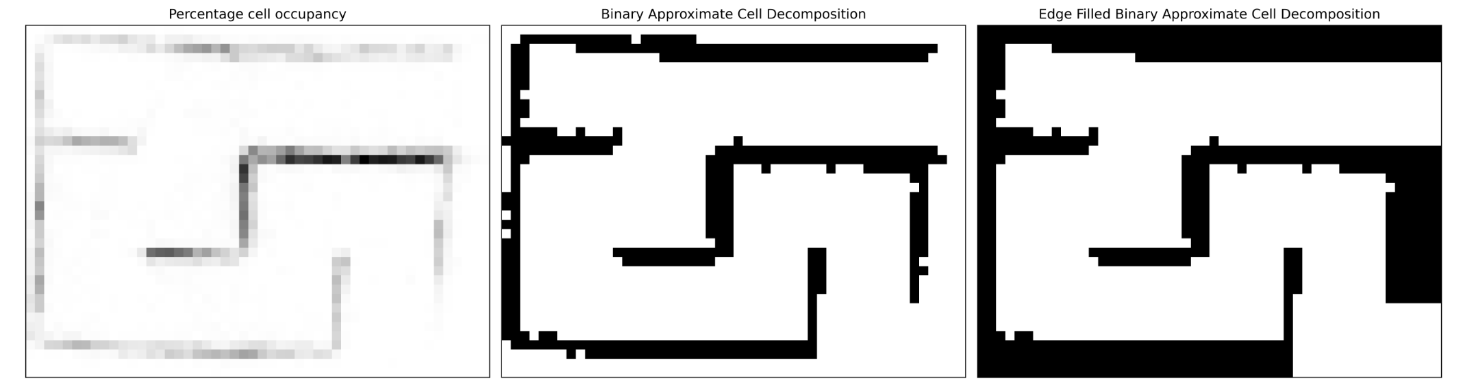
Figure 6: VisualSFM + COLMAP: Results of using the VisualSFM algorithm to do offline Structure from Motion given our sequence of images extracted with additional improved reconstruction results utilizing COLMAP.

Thereafter, we filter the point cloud through a quantiles-based filtering method (Figure 7). This filtered cloud is converted into a topology mapping using approximate cell decomposition (Figure 8).

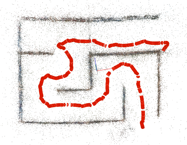
Figure 7: Reconstruction results on the 3D point clouds.

Figure 8: Topological mapping of the reconstructed point clouds. We report (left) the original grid along with the binary approximation through cell decomposition (center), as well as our further improved map (right), filling the edges and removing non-connected points.

This topology mapping is then used to plan a path from the start to the end of the maze using Dijkstra’s algorithm. We first use vanilla Dijkstra, soon realizing the infeasibility of the algorithm with edges weighted by one, see Figure 9.

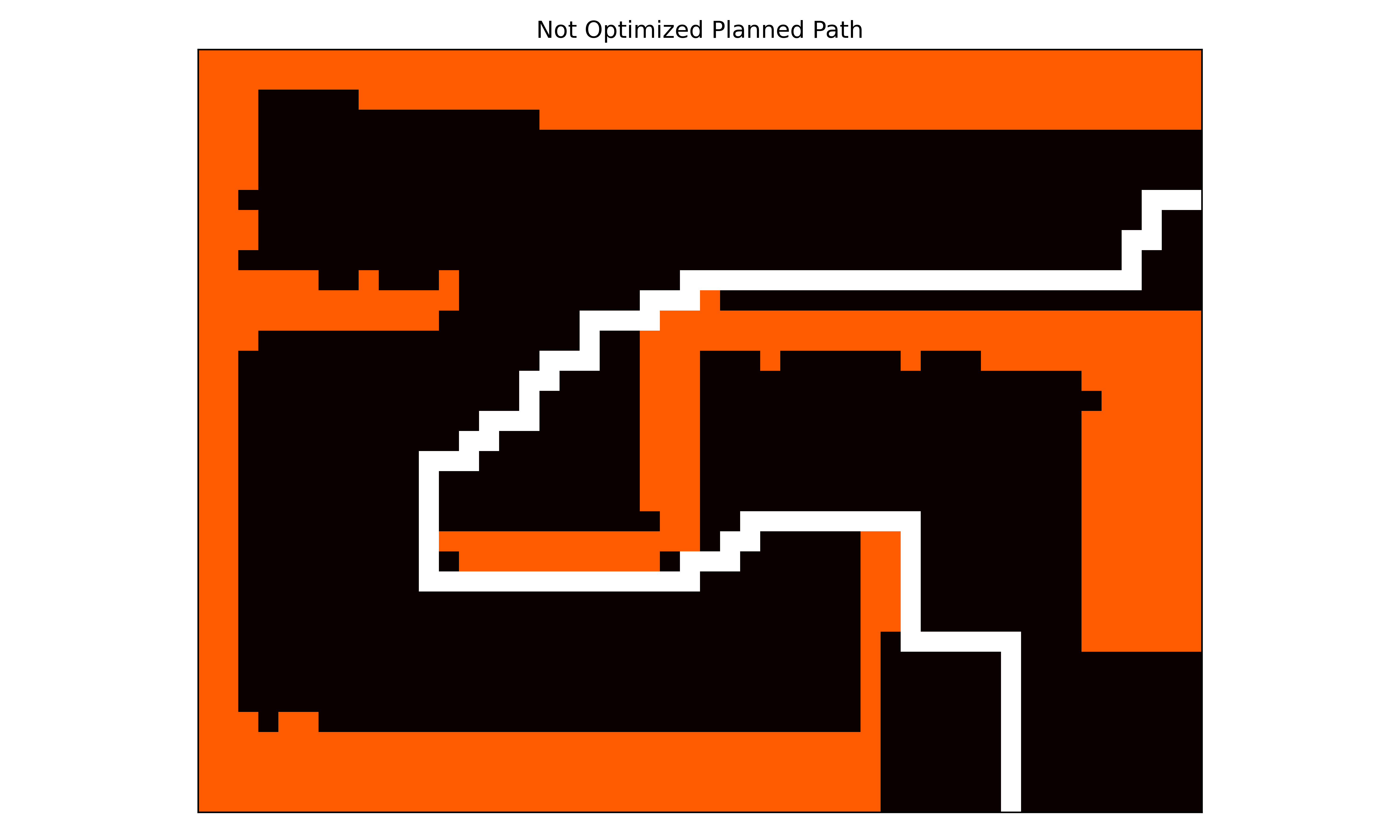
Figure 9: Vanilla Dijkstra with edges weighted by one. The orange pixels indicate occupied cells, black pixels indicate free cells, and white pixels indicate the planned path.

We thus focused on improving the route found using the default Dijkstra a lgorithm by changing it so that we prioritize movement along the center of the roads spanned by the maze. To this effect, we devised a different way to compute the cost for each edge. Instead of setting the cost to one, we added a distance to the occupied cells penalty. This distance penalty should be high if an edge is close to a wall and low if it is far away.

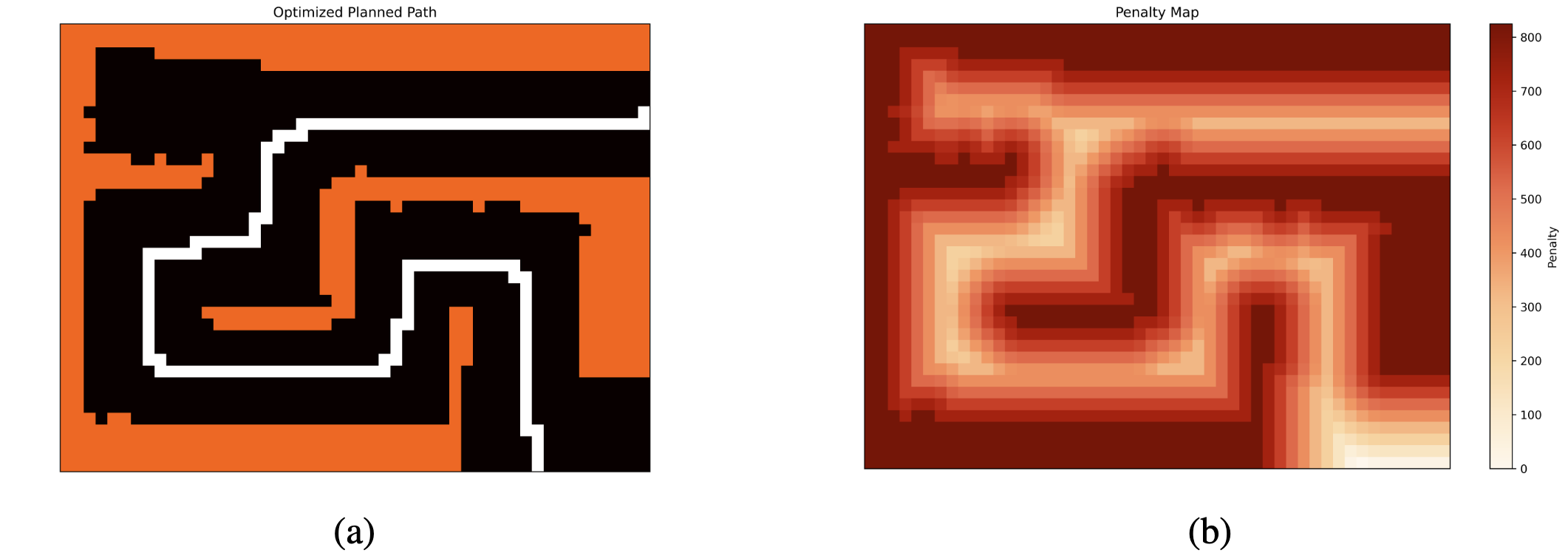
We used scipy.ndimage.distance\_transform\_edt to calculate for each free cell the shortest distance to each occupied cell and scale this by a factor of a hundred. However, adding this distance to each edge would give the opposite effect, as free cells in the middle have a larger distance to occupied cells. We could invert the distance by multiplying it by minus one. However, as Dijkstra tries to find the route with the lowest cost, this leads to negative loops and no solution. Therefore, instead, we took the cell with the largest distance and added this to the distance multiplied by minus one. This resulted in the cell with the largest distance to a free cell not having a penalty and cells close to the wall having the most significant penalty. As our graph is directed, we added the penalty of the outgoing node to each of its edges. For example, if we have the graph A → B. Edge → would get a cost of 1+ penalty(A). The path found using this cost function can be found in Figure 10 (left); this figure clearly shows that the new route follows the middle of the maze, making it considerably easier, more robust, and safer for a robot to follow. Additionally, Figure 10 (right) shows the computed penalty map, showing that our method works since cells in the middle of the path have a low penalty (white) and cells closer to the walls have an increasingly higher penalty (red).

Figure 10: Our optimized planned path (a) that makes use of penalty map (b) in order to calculate the cost of each edge. The orange pixels in (a) indicate occupied cells, the black pixels indicate free cells, and the white pixels indicate the planned path. In (b), the shade of red indicates the applied penalty amount, which increases the closer a cell is to a wall.

Citation

If you use this work, please cite:

@misc{denbraber2025cvar,
  author  = {den Braber, R., and Nulli, M., and Zegveld, D.},
  title   = {Perception, Localization, Planning and Control on RAE Robots},
  howpublished  = {https://matteonulli.github.io/blog/2025/cvar/},
  year    = {2025},
}